MATLAB/Simulink

PCs

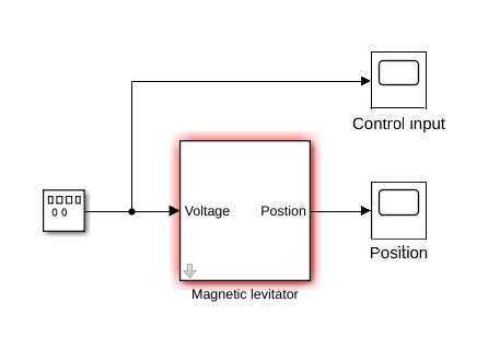
The setups are connected to a lab PC connection by means of a real-time Simulink block (see figure below). This block has one or more input port(s) to which you can use to send an actuation command to the setup (voltage to a motor for instance), and one or more output ports through which you receive the measurements from the setup.

Example of a Simulink diagram containing the real-time block connecting the setup to your lab PC.

An experiment is performed by connecting the real-time Simulink block to relevant other blocks that provide inputs to the system during the experiment.

Before running an experiment, make sure that your calibration is in order, and that you have specified a sampling rate as the variable h in your Matlab workspace.

Template files

The lab PCs contain a folder on the local hard drive, located at C:\Opstellingen\. This folder contains a subfolder for each of the available setups. In these subfolders, you’ll find all the files that are neccesary to build your own experiments. Copy the content of your subfolder to a location in your own user folder (the original subfolders are marked Read-Only).

To perform experiments, start up Matlab (preferably version R2020). A Simulink instance can then be launched by running the command simulink from the command window, or by opening a .slx file. Starting Matlab/Simulink may take a few minutes, be patient.

Your first experiment

• Observe the content of the Simulink file. Open Scope blocks by double-clicking on them.

• Open the settings for the block providing the input to the real-time system. Make sure that the amplitude is zero (or a very small value).

• Define a variable h in your Matlab Workspace, indicating the sampling rate in seconds.

• Click the Run button on the Simulation tab of your Simulink window.

• Observe that you can see the measurements from the sensors in real time in the Scope windows.

Start Matlab (video)

Run Simulink experiment (video)

Run Simulink experiment from the Matlab command line (video)

Run Simulink experiment from a Matlab script (video)

Specifiy a preset input signal for the whole duration of the experiment, and record the observed measurements back to the Matlab Workspace.

Sample Matlab code that was used in the script.

%% Sample code to run experiment from script,
% specifying a fixed input signal and recording the measured
% outputs to a variable in the Workspace for further processing.

clear;clc;

% Sample rate in sec.
h = 0.01;

% Experiment duration in sec. 
% (don't forget to change this in your diagram, see video)
Tsim = 15;

% Time vector (don't forget to transpose with ')
t = [0:h:Tsim]';

% Input vector
amplitude = 0.3;
omega = 1;
u = amplitude * sin(omega * t);

% Variable that goes to Simulink
% (First column: time, Second column: input values)
simin = [t, u]

%% Start experiment
sim rotpentemplate

%% Collect output data
% (make sure that samples are taken every 'h' seconds! in 'To Workspace' block)

% If output type 'Timeseries'
y = simout.Data;

% If output type 'Array' 
% y = simout;

%% Plot data
th1 = y(:, 1);
th2 = y(:, 2);

plot(t, th1, t, th2)
legend('theta_1', 'theta_2')

Calibration

The very first task to complete is to check if the measurements that are coming in from the setup can be trusted. Some setups need calibration, which involves:

Bias

The setups may report biased measurements, some on purpose, others by accident. Fix for this by making sure that the setup is in the desired equilibirium posiiton, and start an experiment with zero input. Record measurements for some time

In every further experiment, subtract the recorded values. Some template Simulink files have a mechanism it built in to the template and some don’t. If you need to, implement the calibration yourself with use of Sum and Constant-blocks.

Measurement Units

For most setups the input values are scaled and saturated between -1 and +1. The output values are not always given in a physically meaningful unit - you could correct for that by multiplying with a constant factor (with use of Gain blocks.

Resources

You’ll need to work with various elements contained within the MATLAB software environment. Examples of places to find documentation are:

• Basics Default MATLAB commands such as plot, load, save, etc.

• Control Systems toolbox Object commands: ss, tf, zpk Time domain and frequency domain analysis: step, bode, nyquist Control design tools: place, acker (be careful with using the Automated Tuning commands!).

• System Identification toolbox (Matlab official)** With functions to pre- or post-process data, estimation and validation models.

• LTI System Identification toolbox With various functions to help you with the use of subspace identification methods.